Recently, on Reddit (of course), someone posted a video talking about how long it would take to fall straight through the center of the earth to the other side. One of the nice parts of the video is that it shows you what the time would be when we account for the actual, non-uniform density of the earth. The video just showed an Excel sheet, though.

I recommend you watch the linked video so you have a good visual of the problem. Once you’ve done that, come on back! In this post I’m going to show you how to solve the problem using Python and a numerical integrator from SciPy.

Basic Kinematics

As a quick refresher, the basics of kinematics (the math of motion through space and time) are that:

Speed is the rate of change of position
Acceleration is the rate of change of speed

All of those are vector quantities (they have direction and magnitude), so you can accelerate by turning, speeding up, or slowing down. Let’s also not forget Newton’s 2nd law:

$F=ma$

Remembering our calculus, the rate of change is called a derivative. The fundamental theorem of calculus tells us that the integral of the derivative of a function is just the function:

$F(x)= \int{f(t) dt}$

$F^{\prime}(x) = f(x)$

That lets us know that we can calculate acceleration (from a model of gravitational force) and just integrate twice with respect to time to find position (the first integration gives us velocity). Therefore, given an initial position and velocity, we can figure out when we reach a new position of interest (like the other side of the Earth) and see how much time passed in the integrator. Here’s what that looks like for velocity:

$v^{\prime} = a = \frac{F}{m}$

$v = \int v^{\prime} = \int a dt$

Equation Setup

Let’s set up the equations of motion for our system in terms of derivatives. Also, keep in mind that we are dealing with vectors, but that they are 1-dimensional vectors (we are only concerned with a line through the earth) whose direction is indicated by a plus or a minus sign. Our convention will be that we start at the ‘top’ of the earth, which is positive. The core is 0, and the ‘bottom’ is negative.

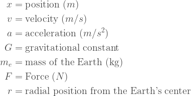
Let’s define some terms first:

$\begin{aligned}x &= \text{position }(m)\\v &= \text{velocity }(m/s)\\a &=\text{acceleration }(m/s^2)\\G &=\text{gravitational constant}\\m_e &=\text{mass of the Earth (kg)}\\F&=\text{Force }(N)\\r&=\text{radial position from the Earth's center}\end{aligned}$

We need to set up our equations in the form of: $F^{\prime} = f$ . This is what that looks like:

$\left[\begin{array}{c}x^{\prime}\\v^{\prime}\end{array}\right]=\left[\begin{array}{c}v\\a\end{array}\right]$

Let’s wrap it up with the integration so we can see where we get position from:

$\left[\begin{array}{c}x\\v\end{array}\right]=\int{\left[\begin{array}{c}x^{\prime}\\v^{\prime}\end{array}\right] dt}$

Uniform Gravity Model

The last thing we have to do is figure out the gravity model. If you look at the equations we’ve set up, only the acceleration term is up to us. The velocity will be solved with integration and we’ll re-input that into the integration at the next time step. The same thing will happen with position, which we need to figure out the force.

The force of gravity is:

$F = G\frac{m_e m}{r^2}$

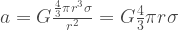
So the acceleration is:

$a = \frac{F}{m} = G\frac{m_e}{r^2}$

Remember from the video that we can ignore the shell of the earth that is ‘above’ us as we fall through the earth. That means that we need $m_e$ as a function of $r$ to finish everything up.

Using a uniform density earth, we have:

$\sigma = \text{Earth's density }(kg/m^3)$

Mass is just volume times density:

$m_e = V\sigma$

$m_e = \frac{4}{3}\pi r^3\sigma$

So finally:

$a= G\frac{\frac{4}{3}\pi r^3\sigma}{r^2}=G\frac{4}{3}\pi r\sigma$

In the code below you’ll see that I don’t factor out the radius like I did here. That’s to keep things consistent for different gravity models. Speaking of which!

Variable Gravity Model

We’ll use a model of the earth’s density from here: http://ds.iris.edu/ds/products/emc-prem/. The density vs radius from the center of the Earth looks like this:

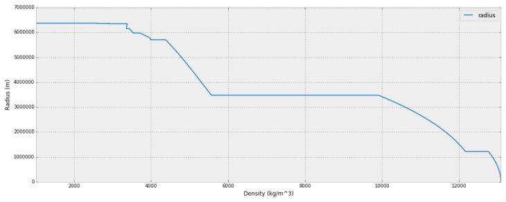
Earth Density Model

We use the same equations as before, it’s just that the mass of the Earth now comes from the addition of all the shells that are below our traveler. The data are in the form of km for the radius and thousands of kg per cubic meter for the density. I convert them to meters and kg/m^3 before using them in the following code.

Now that we know the setup, let’s implement!

Integration in Python

We start by writing our function to return the derivatives to be integrated in a general way, so that we can plug any earth’s mass model in that we want:

# these are all the imports we need:
import numpy as np
import scipy.integrate as integrate
import pandas as pd

def position_model(y, t, accel, accel_inp):
    x = y[0]
    v = y[1]
    r = abs(x)
    a = accel(x, r, *accel_inp)
    return [v, a]

The accel input is a function that calculates the acceleration given the current position x, the absolute position r, and a tuple or list of inputs to the acceleration function. For the acceleration function, we’ll just use the gravity models we’ve made.

Here’s the constant gravity acceleration function:

def constant_accel(x, r, G, rho, radius):
    earth_mass = 4/3 * np.pi * r**3 * rho
    # don't forget to point gravity the right way with sign(x)
    # acceleration is F/m , so ignore the falling object's mass
    a = -sign(x)*G * (earth_mass)/r**2
    return a

For the variable density model, I read in the data:

# load the model using pandas
# the radius is in km, and the density in 1000's of kg/m^3
density_data = pd.read_csv("./PREM_1s.csv", names=['radius', 'density'], usecols=[0, 2])
# convert the units to our base units of meters and kilograms
density_data.radius *= 1000
density_data.density *= 1000
arr_radius = density_data.radius.as_matrix()
arr_density = density_data.density.as_matrix()

Those are inputs to the variable acceleration model:

def variable_accel(x, r, G, density, radius, R):
    # look at all the volume below our depth
    earth_mass = 0
    idx = np.argwhere(radius < r).ravel().min()
    if idx > 0:
        # partial first shell that we are in
        earth_mass = 4/3 * pi * (radius[idx-1]**3 - r**3) * density[idx-1]
    if idx == len(density) - 1:
        # inside the last shell
        earth_mass = 4/3 * pi * (r**3) * density[-1]
    # loop over each shell below us (you could pre-compute these to save some cycles)
    for ix in range(idx, len(density)-1):
        earth_mass += 4/3 * pi * (radius[ix]**3 - radius[ix+1]**3) * density[ix]
    a = -sign(x)*G * (earth_mass)/r**2
    return a

Now that we have our models, we can finally integrate:

# constants
rho = 5514 # kg/m^3
radius = 6371.008 * 1000 # m
G = 6.67408e-11

# generate a bunch of times from 0 to 5 hours, increments at every minute
t = np.linspace(0, 3600, 3600)

# run the integrator on the constant model:
# initial conditions
y0 = [radius, 0]
sol_const = integrate.odeint(position_model, y0, t, args=(constant_accel, (G, rho, radius)))

# run it on the variable model:
# initial conditions
y0 = [d_radius[0], 0]
sol_var = integrate.odeint(position_model, y0, t, args=(variable_accel, (G, arr_density, arr_radius, radius)))

The solution variable is a two-column array where the first column is the position and the second is the velocity. Each row corresponds to the times we defined for the integrator to run over. Plotting and analysis is as simple as plotting the first column (position) vs the times. The time to reach the other side is just the time when we get closest to the negative radius of the earth.

Results for Earth

The integration gives us the following plots for radial position vs. time:

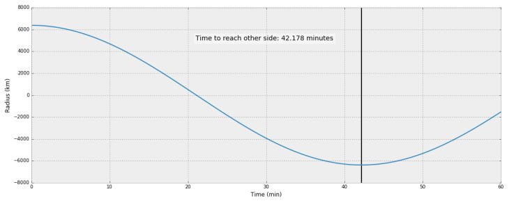
Trajectory with Constant Earth Density

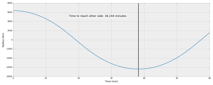
Trajectory with Variable Earth Density

The numbers I got were pretty close to the video’s. Hard to tell whose are more correct, though. I will say that my shell acceleration method is pretty rough, so if you spot an error, let me know!

Results for Mars

I found a paper that had an estimated Martian density profile. That paper is behind a paywall, but if you google the title you’ll find tons of free pdf links. I had to use a digitizer to get the density profile graph, and I also chose the ‘middle’ of the three options. Here’s the table (remember to convert depth to radius for your usage):

depth (m)	density (kg/m^3)
0	3000
50000	3000
51000	3345.225
66808.81	3438.964
1022570	3700.036
1111698	3894.764
1348787	3972.667
1384411	4057.305
1848111	4137.119
1853849	4491.385
1976043	4517.716
1975012	7393.611
33895000	8113.7

Here’s what that looks like:

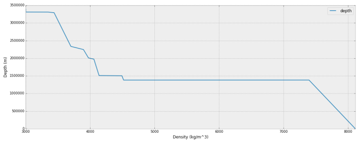
Martian Density Profile

Plugging that in gives us the following Martian core travel profile:

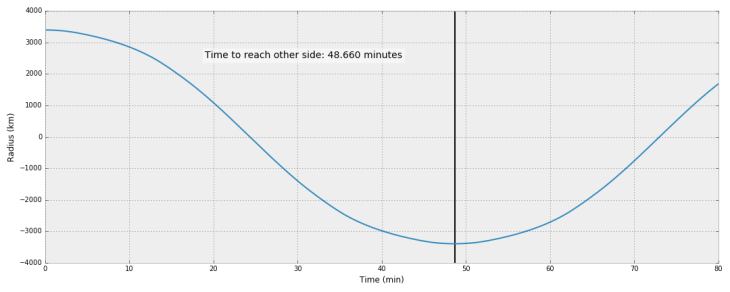
Martian Trajectory with Variable Density

The distance is shorter, but the density is so much less that there isn’t much force to pull you faster.The time under a constant density assumption is only 50 minutes.

Finally, here’s all of them on one plot:

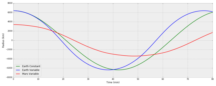
Our Planet Base-Jumper’s Travels

Primed

Data, engineering, and other stuff

Falling Through the Earth (and Mars)

Basic Kinematics

Equation Setup

Uniform Gravity Model

Variable Gravity Model

Integration in Python

Results for Earth

Results for Mars

Leave a comment Cancel reply

Basic Kinematics

Equation Setup

Uniform Gravity Model

Variable Gravity Model

Integration in Python

Results for Earth

Results for Mars

Share this:

Related

Leave a comment Cancel reply